Constant Volume Energy Minimization Tutorial#

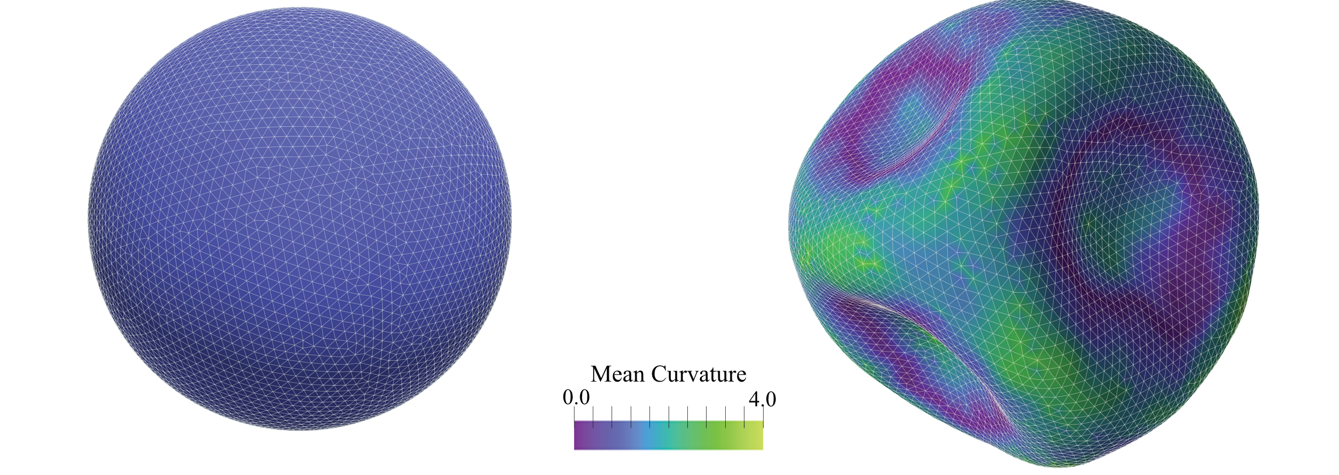
Figure: (Left) Initial configuration of a vesicle with unit radius comprising $N=6281$ vertices. The vesicle is subjected to a strain by increasing the edge rest length as $l_0 = (1+epsilon) left<l_eright>$, where $epsilon = 0.1$ and $left<l_eright>$ denotes the average edge length of the mesh. As a result, the vesicle buckles, leading to surface wrinkles, as depicted in (Right). The colour bar indicates the local mean curvature. The final shape of the vesicle, after energy minimization under volume constraint, is obtained using the FIRE method#
Introduction#
In this tutorial, you will learn how to use PyMembrane to perform constant volume energy minimization of a closed elastic vesicle. This example minimizes the total elastic energy subject to the volume constraint, following the given code.
Requirements#
Python
NumPy
Matplotlib
SciencePlots
Running the Code#
Note
This tutorial assumes that you have already installed PyMembrane. If not, please refer to the installation instructions in the installation section.
Save the provided code as
minimizer.pyDownload
verticesandfaces.Run the script by executing:
python minimization.py --snapshots N_SNAPSHOTS --max_iter MAX_ITER
PyMembrane Implementation#
#import the code
import pymembrane as mb
import numpy as np
from pprint import pprint
import argparse
import matplotlib.pyplot as plt
import matplotlib.ticker as ticker
import scienceplots
plt.style.use(['science'])


### Parse arguments
## Now we want to have X snapshots every X steps each
parser = argparse.ArgumentParser(description="Please provide: snapshots and run_steps")
## Add arguments for snapshots and run_steps
parser.add_argument("--snapshots", type=int, required=True, help="Number of snapshots")
parser.add_argument("--max_iter", type=int, required=True, help="Number of iteration steps")

user_args = parser.parse_args()
# Access the parsed arguments
snapshots = user_args.snapshots
max_iter = user_args.max_iter

vertex_file = 'vertices_R1.0_l01.inp'
face_file = 'faces_R1.0_l01.inp'

#create a system
box = mb.Box(40,40,40)
system = mb.System(box)
system.read_mesh_from_files(files={'vertices':vertex_file, 'faces':face_file})

#save the mesh to display
#create dumper
dump = system.dumper
dump.vtk("initial mesh", False)


#add the evolver class where the potentials and integrators are added
evolver = mb.Evolver(system)

# first we need to know the edge length to move it appropriate:
compute = system.compute
edge_lengths = compute.edge_lengths()
avg_edge_length= np.mean(edge_lengths)
print("[Initial] avg_edge_length = ", avg_edge_length)

#add the potentials in this case we will add bending and stretching
# stretching
k = str(400.0)
# add some strain into the edges
l0 = str(1.1*avg_edge_length)
#l0 = str(avg_edge_length)
evolver.add_force("Mesh>Harmonic", {"k":{"0":k},
                                    "l0":{"0":l0}})

# limit potential
lmin = str(0.5*np.min(edge_lengths))
lmax = str(2.0*np.max(edge_lengths))
evolver.add_force("Mesh>Limit", {"lmin":{"0":lmin},
                                "lmax":{"0":lmax}})

# bending potential
kappa = str(1.0)
evolver.add_force("Mesh>Bending>Dihedral", {"kappa":{"0":kappa}})

# Add the minimizer
evolver.add_minimizer("Mesh>Fire", {"dt": str(1e-2),
                                    "max_iter": str(max_iter),
                                    "ftol": str(1e-2),
                                    "etol": str(1e-4)})
pprint(evolver.get_minimizer_info())

# Add volume constraint
initial_volume = compute.volume()
evolver.add_constraint("Mesh>Volume", {"V": str(initial_volume),
                                    "max_iter": str(10000),
                                    "tol":str(1e-5)})

# Randomize the mesh to avoid initial freezing
rnd_move = 0.5*np.std(edge_lengths)/6.0
vertices = system.vertices
for vertex in vertices:
    vertex.r.x += np.random.uniform(-rnd_move, rnd_move)
    vertex.r.y += np.random.uniform(-rnd_move, rnd_move)
    vertex.r.z += np.random.uniform(-rnd_move, rnd_move)
system.vertices = vertices

## Compute the initial energy
min_energy = snapshots*[None]
min_energy[0] = 100.0*compute.energy(evolver)['edges']/system.Numedges
print("[Initial] energy:{} x 10^-2 volume:{}".format(min_energy[0], compute.volume()))

# Minimize
dump.vtk("minimization_t0")
for snapshot in range(1, snapshots):
    evolver.minimize()
    dump.vtk("minimization_t{}".format(snapshot))
    min_energy[snapshot] =  100.0*compute.energy(evolver)['edges']/system.Numedges
    print("[{}] energy:{} x 10^-2 volume:{}".format(snapshot, min_energy[snapshot], compute.volume()))
pprint(evolver.get_minimizer_info())

# Compute the final volume
energy = compute.energy(evolver)
print("[Final] energy:{} x 10^-2 volume:{}".format(min_energy[snapshots-1], compute.volume()))
final_volume = compute.volume()
print("volume difference: {}".format(final_volume-initial_volume))

dump.txt("minimized")

fig, ax = plt.subplots(figsize=(3.3,3.3))
ax.plot(min_energy, 'o-')
ax.set_xlabel(r"$Steps$", fontsize=10, labelpad = 2.5)
ax.set_ylabel(r"$Energy/NumEdges \times 10^{-2}$", fontsize=11, labelpad = 2.5)
ax.tick_params(axis='x', labelsize=8, pad = 4)
ax.tick_params(axis='y', labelsize=8, pad = 4)
ax.ticklabel_format(useMathText=True)
ax.xaxis.set_major_formatter(ticker.ScalarFormatter())
ax.yaxis.set_major_formatter(ticker.ScalarFormatter())
plt.tight_layout()
plt.savefig("energy.svg", dpi=400)
Description#
The code begins by importing required libraries and parsing command-line arguments for the number of snapshots and iteration steps.
Create the System: A system is created with a specified box size, and the mesh is read from files.
Initial Mesh: The initial mesh is saved for visualization.
Evolver and Potentials: An Evolver class is created, where potentials and integrators are added. The stretching and bending potentials are defined based on the provided parameters.
Minimizer and Constraints: The minimizer is added, and the volume constraint is set. The mesh can be randomized to avoid initial freezing.
Minimization: The code runs the minimization algorithm, saving snapshots of the mesh and computing energy at each step.
Results and Visualization: The code prints the final energy and volume, and a plot of the energy is saved.
Final Remarks#
This example demonstrates the power of PyMembrane in handling complex elastic vesicle simulations. The ability to perform energy minimization while maintaining a constant volume is a crucial aspect of simulating biological systems. Modify the parameters and potentials to explore different behaviors and study various physical phenomena.
Please refer to the references cited in the text for detailed methodologies and theoretical background.