Caspar-Klug Thin Shells Buckling#

initial mesh

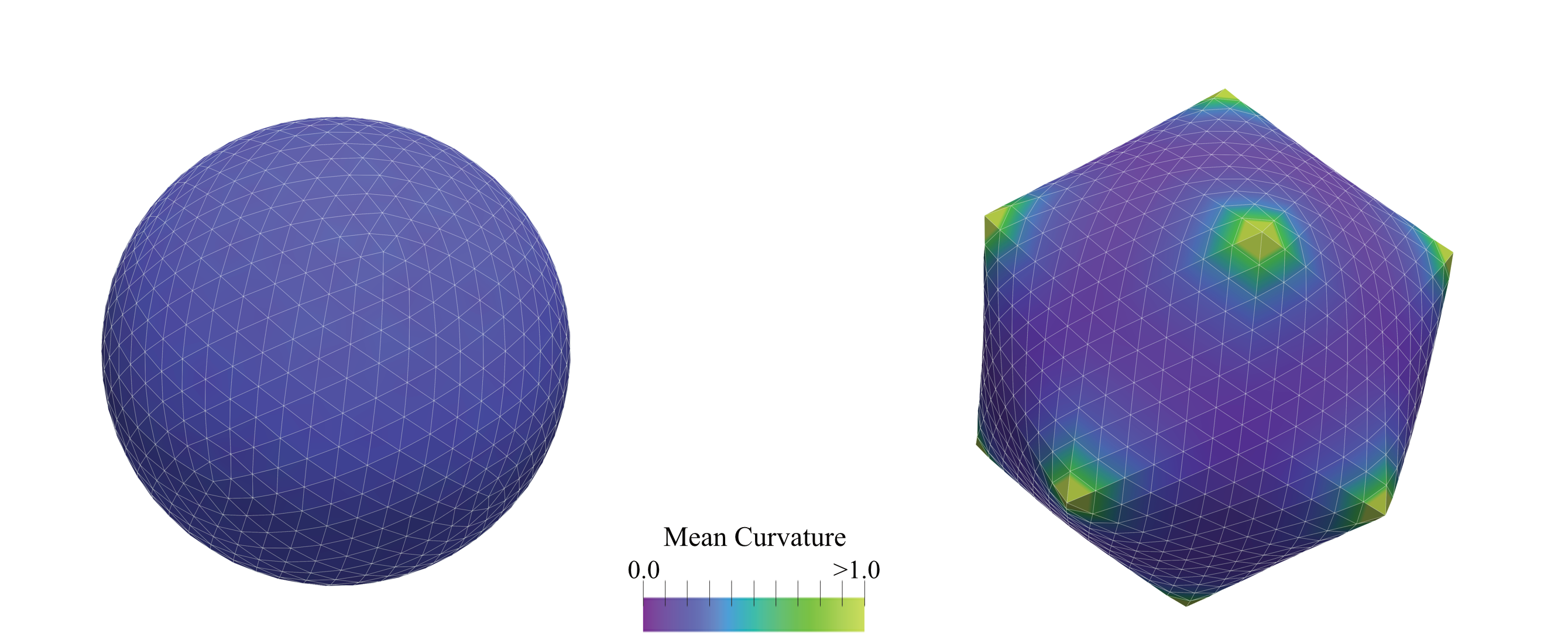
Figure: Snapshots of a Monte Carlo simulation of an icosahedral closed shell, representing a virus with $T=108$ ($(p,q)=(6,6)$), according to the Caspar-Klug classification~cite{caspar1962physical}. The material parameters are chosen such that the F"oppl-von K'arm'an number is $gamma approx 400$. (Left) The sphere with 12 5-fold defects at the corners of an icosahedron prior to buckling; (Right) a buckled, faceted structure. The colour bar represents the local mean curvature of the mesh.#

Introduction#

This tutorial demonstrates how PyMembrane can be used to understand the shape of certain types of viruses through the mechanics of thin shells. Caspar and Klug showed that shell proteins in viruses form an icosahedral triangulation of a sphere, resulting in at least 12 pentavalent sites that are +1 disclinations. These can buckle if the Föppl-von Kármán number is sufficiently large, explaining why smaller viruses are spherical and larger ones are faceted.

Requirements#

Note

This tutorial assumes that you have already installed PyMembrane. If not, please refer to the installation instructions in the installation section.

  • Python

  • NumPy

  • Matplotlib

  • SciencePlots

Running the Code#

  1. Save the provided code as buckling.py.

  2. Download vertices, faces.

  3. Run the script by executing:

    python buckling.py --snapshots N_SNAPSHOTS --run_steps N_RUN_STEPS
    

PyMembrane Implementation#

First, you’ll need to import the PyMembrane library and other necessary components. Then, parse the required arguments, such as snapshots, run_steps, and the spring constant, k=350.0.

import pymembrane as mb
import numpy as np
from pprint import pprint
import argparse
import matplotlib.pyplot as plt
import matplotlib.ticker as ticker
import scienceplots
plt.style.use(['science'])


### Parse arguments
## Now we want to have X snapshots every X steps each
parser = argparse.ArgumentParser(description="Please provide: snapshots and run_steps")
## Add arguments for snapshots and run_steps
parser.add_argument("--snapshots", type=int, required=True, help="Number of snapshots")
parser.add_argument("--run_steps", type=int, required=True, help="Number of run steps")

user_args = parser.parse_args()
# Access the parsed arguments
snapshots = user_args.snapshots
run_steps = user_args.run_steps

#create a system
box = mb.Box(4,4,4)

system = mb.System(box)

#check if the box is loaded correctly
print(system.box)

#read the mesh
vertex_file = 'vertices.dat'
face_file = 'faces.dat'
system.read_mesh_from_files(files={'vertices':vertex_file, 'faces':face_file})


#save the mesh to display
#create dumper
dump = system.dumper
dump.vtk("initial mesh", False)


#add the evolver class where the potentials and integrators are added
evolver = mb.Evolver(system)


#add the potentials in this case we will add bending and stretching
# stretching
k = str(350.0)
l0 = str(1.0)
evolver.add_force("Mesh>Harmonic", {"k":{"0":k},
                                    "l0":{"0":l0}})

# limit potential
lmin = str(0.7)
lmax = str(1.3)
evolver.add_force("Mesh>Limit", {"lmin":{"0":lmin},
                                "lmax":{"0":lmax}})
# bending potential
kappa = str(1.0)
evolver.add_force("Mesh>Bending>Dihedral", {"kappa":{"0":kappa}})

#Print the loaded forces
pprint(evolver.get_force_info())


# vertex move:
# first we need to know the edge length to move it appropriate:
compute = system.compute
edge_lengths = compute.edge_lengths()
avg_edge_length= np.mean(edge_lengths)
print("[Initial] avg_edge_length = ", avg_edge_length)

#add the monte carlo integrator
evolver.add_integrator("Mesh>MonteCarlo>vertex>move", {"dr":"0.008"})


## Compute the initial energy
mc_energy = snapshots*[None]
mc_energy[0] = 100.0*compute.energy(evolver)['edges']/system.Numedges
print("[Initial] energy = {} x 10^-2".format(mc_energy[0]))

dump.vtk("sphere_t0")
for snapshot in range(1, snapshots):
    for temperature in [1e-3, 1e-5, 1e-7, 0.0]: #using heating and cooling cycles
        evolver.set_global_temperature(str(temperature))
        evolver.evolveMC(steps=run_steps)
    dump.vtk("sphere_t" + str(snapshot*run_steps))
    mc_energy[snapshot] =  100.0*compute.energy(evolver)['edges']/system.Numedges
    print("[{}] energy = {} x 10^-2".format(snapshot,  mc_energy[snapshot]))

dump.vtk('final_mesh')

edge_lengths = compute.edge_lengths()
avg_edge_length= np.mean(edge_lengths)
print("[Final] avg_edge_length = ", avg_edge_length)

energy = compute.energy(evolver)
print("[Final] energy = ", mc_energy[snapshots-1])

dump.txt("pentagon")

fig, ax = plt.subplots(figsize=(3.3,3.3))
ax.plot(mc_energy, 'o-')
ax.set_xlabel(r"$MC steps$", fontsize=10, labelpad = 2.5)
ax.set_ylabel(r"$Energy/NumEdges \times 10^{-2}$", fontsize=11, labelpad = 2.5)
ax.tick_params(axis='x', labelsize=8, pad = 4)
ax.tick_params(axis='y', labelsize=8, pad = 4)
ax.ticklabel_format(useMathText=True)
ax.xaxis.set_major_formatter(ticker.ScalarFormatter())
ax.yaxis.set_major_formatter(ticker.ScalarFormatter())
plt.tight_layout()
plt.savefig("energy.svg", dpi=400)

Result and Interpretation#

This example highlights the capability of PyMembrane in handling closed membranes, specifically in understanding the mechanics of thin shells. Follow the code snippets provided to configure and run the simulation.

Attached Files#

Python script: Monte Carlo Sphere

Input files: vertices, faces

References#

[Lidmar03]
  1. Lidmar, L. Mirny, D. R. Nelson, Virus shapes and buckling transitions in spherical shells, Physical Review E 68 (2003)

051910

Note#

Please refer to the PyMembrane documentation for more specific details about classes and methods used in this tutorial. Feel free to modify parameters and observe how they influence the results.