Periodic Boundary#
In many problems, probing finite-size effects is crucial, especially when modelling long-wavelength properties or when long-range interactions are present. Periodic boundary conditions are often used to replicate an infinite system by replicating the simulation box. This example models wrinkling in a periodic thin sheet subject to uniaxial compression.
What This Example Demonstrates#
This example loads the packaged mesh files vertices.dat and faces.dat
from the periodic example data set, constructs a periodic box, applies
stretching, limiting, and dihedral bending forces, and evolves the mesh with a
Brownian vertex-move integrator while the box is compressed along one
direction. It writes initial_mesh.vtk and a sequence of
periodic_t*.vtk files that can be inspected in ParaView or any other tool
that reads legacy VTK polygon data. --quick keeps the same physical setup
but reduces the number of snapshots and integration steps.
How to Run#
After installing PyMembrane, run the packaged example from any working directory:
python -m pymembrane.examples.periodic --quick
To keep output files in a separate directory:
python -m pymembrane.examples.periodic --quick --output-dir results
Inputs#
packaged mesh files:
vertices.datandfaces.datoutput directory: current working directory unless
--output-diris used
Model Ingredients#
mesh: periodic triangulated sheet mirrored under
docs/examples/periodicforces:
Mesh>Harmonic,Mesh>Limit,Mesh>Bending>Dihedralintegrator:
Mesh>Brownian>vertex>moveboundary condition: periodic box in all three directions
Expected Output#
initial_mesh.vtkperiodic_t0.vtkadditional
periodic_t*.vtksnapshotsoutput format: legacy ASCII
.vtk
Quick Mode#
Quick mode keeps the same model and mesh, but reduces the number of snapshots and Brownian dynamics steps.
Minimal Workflow#
The packaged script follows the standard PyMembrane workflow:
from math import sqrt
import pymembrane as mb

box = mb.Box(sqrt(3.0) * 29, 50.0, 50.0, True, True, True)
system = mb.System(box)
system.read_mesh_from_files(files={"vertices": "vertices.dat", "faces": "faces.dat"})
system.enforce_boundaries()

evolver = mb.Evolver(system)
evolver.add_force("Mesh>Harmonic", {"k": {"0": "100.0"}, "l0": {"0": "1.0"}})
evolver.add_force("Mesh>Limit", {"lmin": {"0": "0.7"}, "lmax": {"0": "1.3"}})
evolver.add_force("Mesh>Bending>Dihedral", {"kappa": {"0": "1.0"}})
evolver.add_integrator("Mesh>Brownian>vertex>move", {"seed": "202208"})
evolver.set_time_step("2e-3")
evolver.set_global_temperature("1e-4")
evolver.evolveMD(steps=10)
system.dumper.vtk("output", periodic=True)
Results#
The periodic structure shows clear wrinkles, indicative of the system’s response to compression. You can observe the geometry in the generated VTK files.
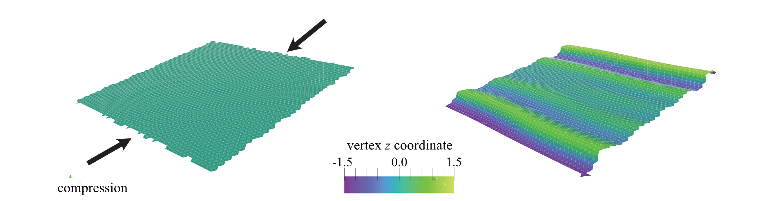
Figure: The periodic structure shows clear wrinkles on the surface.#